Example of training time reduction for a classifier
May 10, 2022 Shoichiro Yokotani, Application Development Expert AI Platform division
In machine learning algorithms, supervised learning can be categorized into two types: regression and classification. In this article, we will take the latter, classification, as an example and run a sample using the Frovedis learning algorithm. We will also compare the time required for learning between the Frovedis version and the scikit-learn version.
Classifiers are applied to datasets with discrete output y for many input variables. For example, the Credit Card Fraud Detection dataset used in this study has 29 different features with binary output y, such as Not Fraud and Fraud. We will use this data set to make a two-class decision using a machine learning algorithm.
Typical machine learning algorithms for classifications include logistic regression, linear support vector machines, random forests as an ensemble method of classification trees and classification trees, and gradient boosting classification trees. In this column, we will focus on two-class classification using classification trees and gradient boosting classification trees.
Gradient boosting decision trees can be used for class classification. scikit-learn version of gradient boosting decision trees does not perform parallel processing, but Frovedis version processes each decision tree creation in parallel, so it is expected to reduce training time compared to scikit-learn on very large datasets. The Frovedis version is expected to reduce training time compared to scikit-learn on very large datasets.
Two-class classification using classification trees and gradient boosting classification trees (training time comparison between scikit-learn version and Frovedis version)
Dataset: Credit Card Fraud Detection https://www.kaggle.com/mlg-ulb/creditcardfraud
Loading the dataset
in [1]:
|
import numpy as np import pandas as pd df = pd.read_csv('../../data/classify/creditcard.csv') class_names = {0:'Not Fraud', 1:'Fraud'} print(df.Class.value_counts().rename(index = class_names)) data_features = df.drop(['Time', 'Class'], axis=1).values data_target = df['Class'].values |
Not Fraud 284315
Fraud 492
Name: Class, dtype: int64
in [2]:
| df.drop(['Time', 'Class'], axis=1).head() |
| V1 | V2 | V3 | V4 | V5 | V6 | V7 | V8 | V9 | V10 | ... | |
|---|---|---|---|---|---|---|---|---|---|---|---|
| 0 | -1.359807 | -0.072781 | 2.536347 | 1.378155 | -0.338321 | 0.462388 | 0.239599 | 0.098698 | 0.363787 | 0.090794 | ... |
| 1 | 1.191857 | 0.266151 | 0.166480 | 0.448154 | 0.060018 | -0.082361 | -0.078803 | 0.085102 | -0.255425 | -0.166974 | ... |
| 2 | -1.358354 | -1.340163 | 1.773209 | 0.379780 | -0.503198 | 1.800499 | 0.791461 | 0.247676 | -1.514654 | 0.207643 | ... |
| 3 | -0.966272 | -0.185226 | 1.792993 | -0.863291 | -0.010309 | 1.247203 | 0.237609 | 0.377436 | -1.387024 | -0.054952 | ... |
| 4 | -1.158233 | 0.877737 | 1.548718 | 0.403034 | -0.407193 | 0.095921 | 0.592941 | -0.270533 | 0.817739 | 0.753074 | ... |
| V20 | V21 | V22 | V23 | V24 | V25 | V26 | V27 | V28 | Amount | ||
| 0 | 0.251412 | -0.018307 | 0.277838 | -0.110474 | 0.066928 | 0.128539 | -0.189115 | 0.133558 | -0.021053 | 149.62 | |
| 1 | -0.069083 | -0.225775 | -0.638672 | 0.101288 | -0.339846 | 0.167170 | 0.125895 | -0.008983 | 0.014724 | 2.69 | |
| 2 | 0.524980 | 0.247998 | 0.771679 | 0.909412 | -0.689281 | -0.327642 | -0.139097 | -0.055353 | -0.059752 | 378.66 | |
| 3 | -0.208038 | -0.108300 | 0.005274 | -0.190321 | -1.175575 | 0.647376 | -0.221929 | 0.062723 | 0.061458 | 123.50 | |
| 4 | 0.408542 | -0.009431 | 0.798278 | -0.137458 | 0.141267 | -0.206010 | 0.502292 | 0.219422 | 0.215153 | 69.99 |
in [3]:
|
from sklearn.model_selection import train_test_split np.random.seed(123) X_train, X_test, y_train, y_test = train_test_split(data_features, data_target, train_size=0.70, test_size=0.30, random_state=1) |
Learning and inference with the Frovedis version of Classification Trees
in [4]:
|
import os, time from frovedis.exrpc.server import FrovedisServer from frovedis.mllib.tree import DecisionTreeClassifier as frovDecisionTreeClassifier FrovedisServer.initialize("mpirun -np 6 {}".format(os.environ['FROVEDIS_SERVER'])) fdtc = frovDecisionTreeClassifier(max_depth=8) t1 = time.time() fdtc.fit(X_train, y_train) t2 = time.time() print ("train time: {:.3f} sec".format(t2-t1)) |
Displaying inference results
in [5]:
|
from sklearn.metrics import confusion_matrix from sklearn.metrics import f1_score, recall_score pred = fdtc.predict(X_test) cmat = confusion_matrix(y_test, pred) tpos = cmat[0][0] fneg = cmat[1][1] fpos = cmat[0][1] tneg = cmat[1][0] f1Score = round(f1_score(y_test, pred), 2) recallScore = round(recall_score(y_test, pred), 2) print('confusion matrix:') print(cmat) print('Accuracy: '+ str(np.round(100*float(tpos+fneg)/float(tpos+fneg + fpos + tneg),2))+'%') print("Recall : {recall_score}".format(recall_score = recallScore)) print("F1 Score : {f1_score}".format(f1_score = f1Score)) FrovedisServer.shut_down() |
[[85292 16]
[ 34 101]]
Accuracy: 99.94%
Recall : 0.75
F1 Score : 0.8
Learning with scikit-learn version of classification tree
in [6]:
|
import os, time from sklearn.tree import DecisionTreeClassifier as skDecisionTreeClassifier sdtc = skDecisionTreeClassifier(max_depth=8) t1 = time.time() sdtc.fit(X_train, y_train) t2 = time.time() print ("train time: {:.3f} sec".format(t2-t1)) |
Displaying inference results
in [7]:
|
pred = sdtc.predict(X_test) cmat = confusion_matrix(y_test, pred) tpos = cmat[0][0] fneg = cmat[1][1] fpos = cmat[0][1] tneg = cmat[1][0] f1Score = round(f1_score(y_test, pred), 2) recallScore = round(recall_score(y_test, pred), 2) print('confusion matrix:') print(cmat) print('Accuracy: '+ str(np.round(100*float(tpos+fneg)/float(tpos+fneg + fpos + tneg),2))+'%') print("Recall : {recall_score}".format(recall_score = recallScore)) print("F1 Score : {f1_score}".format(f1_score = f1Score)) |
[[85295 13]
[ 37 98]]
Accuracy: 99.94%
Recall : 0.73
F1 Score : 0.8
Training and inference with Frovedis version of gradient boosting classification tree
in [8]:
|
from frovedis.mllib.ensemble import GradientBoostingClassifier FrovedisServer.initialize("mpirun -np 6 " + os.environ["FROVEDIS_SERVER"]) fgb = GradientBoostingClassifier(n_estimators=500, learning_rate= 0.01) t1 = time.time() fgb.fit(X_train, y_train) t2 = time.time() print ("train time: {:.3f} sec".format(t2-t1)) |
Displaying inference results
in [9]:
|
pred = fgb.predict(X_test) cmat = confusion_matrix(y_test, pred) tpos = cmat[0][0] fneg = cmat[1][1] fpos = cmat[0][1] tneg = cmat[1][0] f1Score = round(f1_score(y_test, pred), 2) recallScore = round(recall_score(y_test, pred), 2) print('confusion matrix:') print(cmat) print('Accuracy: '+ str(np.round(100*float(tpos+fneg)/float(tpos+fneg + fpos + tneg),2))+'%') print("Recall : {recall_score}".format(recall_score = recallScore)) print("F1 Score : {f1_score}".format(f1_score = f1Score)) FrovedisServer.shut_down() |
[[85300 8]
[ 35 100]]
Accuracy: 99.95%
Recall : 0.74
F1 Score : 0.82
Learning and inference with scikit-learn's version of gradient boosting classification trees
in [10]:
|
from sklearn.ensemble import GradientBoostingClassifier sgb = GradientBoostingClassifier(n_estimators=500, learning_rate=0.01) t1 = time.time() sgb.fit(X_train, y_train) t2 = time.time() print ("train time: {:.3f} sec".format(t2-t1)) |
Displaying inference results
in [11]:
|
pred = sgb.predict(X_test) cmat = confusion_matrix(y_test, pred) tpos = cmat[0][0] fneg = cmat[1][1] fpos = cmat[0][1] tneg = cmat[1][0] f1Score = round(f1_score(y_test, pred), 2) recallScore = round(recall_score(y_test, pred), 2) print('confusion matrix:') print(cmat) print('Accuracy: '+ str(np.round(100*float(tpos+fneg)/float(tpos+fneg + fpos + tneg),2))+'%') print("Recall : {recall_score}".format(recall_score = recallScore)) print("F1 Score : {f1_score}".format(f1_score = f1Score)) |
[[85297 11]
[ 37 98]]
Accuracy: 99.94%
Recall : 0.73
F1 Score : 0.8
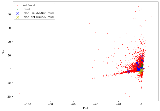
Displaying Inference Results on Frovedis Version of Gradient Boosting Classification Trees by PCA Dimensional Compression
in [12]:
|
from sklearn.preprocessing import StandardScaler scaler = StandardScaler() scaler.fit(X_test) X_scaled = scaler.transform(X_test) from frovedis.mllib.ensemble import GradientBoostingClassifier from frovedis.decomposition import PCA FrovedisServer.initialize("mpirun -np 6 " + os.environ["FROVEDIS_SERVER"]) from frovedis.mllib.ensemble import GradientBoostingClassifier fgb = GradientBoostingClassifier(n_estimators=500, learning_rate=0.01) fgb.fit(X_train, y_train) pca = PCA(n_components=2) pca.fit(X_scaled) X_pca = pca.transform(X_scaled) data = {'PCA1': X_pca[:,0], 'PCA2': X_pca[:,1], 'Target': y_test, 'Test': fgb.predict(X_test)} df = pd.DataFrame(data) df.head() |
| PCA1 | PCA2 | Target | Test | |
|---|---|---|---|---|
| 0 | 0.587710 | -0.102335 | 0 | 0 |
| 1 | 0.510780 | -0.442828 | 0 | 0 |
| 2 | 0.466657 | -0.192914 | 0 | 0 |
| 3 | 0.354354 | 0.037564 | 0 | 0 |
| 4 | 0.471092 | -0.166892 | 0 | 0 |
in [13]:
|
import matplotlib.pyplot as plt df_0 = df[(df.Target==0) & (df.Test==0)] df_1 = df[(df.Target==1) & (df.Test==1)] df_test_0 = df[(df.Target==1) & (df.Test==0)] df_test_1 = df[(df.Target==0) & (df.Test==1)] plt.figure(figsize=(10,7)) plt.scatter(df_0['PCA1'], df_0['PCA2'], color='r', s=2, label='Not Fraud') plt.scatter(df_1['PCA1'], df_1['PCA2'], color='g', s=2, label='Fraud') plt.scatter(df_test_0['PCA1'], df_test_0['PCA2'], color='b', marker='x', s=100, label='False: Fraud->Not Fraud') plt.scatter(df_test_1['PCA1'], df_test_1['PCA2'], color='y', marker='x', s=100, label='False: Not Fraud->Fraud') plt.xlabel("PC1") plt.ylabel('PC2') plt.legend() plt.show() |
in [14]:
| FrovedisServer.shut_down() |
| Learning algorithms | Frovedis (sec) | scikit-learn (sec) | Ratio |
|---|---|---|---|
| ClassificationTrees | 0.26 | 7.81 | x30.0 |
| Gradient boosting | 16.84 | 1398.77 | x83.1 |
The optimization and cross-validation of large data sets by iteratively training with varying machine learning parameters can be time consuming in many cases. In cases where data with new characteristics are frequently added, time-consuming re-training is repeated.
By using Frovedis' parallelized algorithms on SX-Aurora TSUBASA, high performance training models can be prepared frequently and quickly, reducing the cost of system development and maintenance.