Regression analysis using gradient boosting regression tree
Nov 1, 2021, Shoichiro Yokotani, Application Development Expert, AI Platform division
Machine learning algorithms are generally categorized as supervised learning and unsupervised learning. Supervised learning is used for analysis to get predictive values for inputs. "Supervised" learning requires data combinations of inputs and outputs. Learning processes are performed based on these combinations, and the output data is predicted from the input data using the learning results.
In addition, supervised learning is divided into two types: regression analysis and classification. Regression analysis uses machine learning to find the parameters that determine the relationship in order to predict the output y from the input x. Classification is an analysis of a dataset with discrete output y. The output y does not have to be continuous as in regression analysis. For example, it is used to determine the possibility of purchasing a product based on customer information (annual income, family structure, age, address, etc.).
In addition to regression analysis and classification, there are various machine learning algorithms based on mathematical and statistical methods. Depending on the nature of the dataset and the complexity of the model, it is necessary to determine which algorithm is best for the analysis. It is important to fully understand and select the characteristics of each algorithm.
This column introduces the following analysis methods.
(1) Supervised learning, regression analysis.
(2) Machine learning algorithm, gradient boosting regression tree.
Gradient boosting regression trees are based on the idea of an ensemble method derived from a decision tree. The decision tree uses a tree structure. Starting from tree root, branching according to the conditions and heading toward the leaves, the goal leaf is the prediction result. This decision tree has the disadvantage of overfitting test data if the hierarchy is too deep. As a means to prevent this overfitting, the idea of the ensemble method is used for decision trees. This technique uses a combination of multiple decision trees rather than simply a single decision tree. Random forest and gradient boosting are known as typical algorithms.
Random forests create multiple decision trees by splitting a dataset based on random numbers. It prevents overfitting by making predictions for all individual decision trees and averaging the regression results.
Gradient boosting, on the other hand, is a technique for repeatedly adding decision trees so that the next decision tree corrects the previous decision tree error. Compared to Random forest, the results are more sensitive to parameter settings during training. However, with the correct parameter settings, you will get better test results than random forest.
Both random forest and gradient boosting are implemented in scikit-learn. Both learning algorithms can be used in Frovedis as well. There is no parallel processing in the scikit-learn version of Gradient Boosting. However, Frovedis can process individual decision tree creations in parallel. Learning time can be reduced compared to scikit-learn for very large data sets.
This column presents a Gradient Boosting Regression Analysis Demonstration with Frovedis.
This demo uses Kaggle's used car sales price dataset.
The procedure is as follows.
--Integrating data stored in CSV by brand into one table
--Selecting the year of manufacture, mileage, and displacement of the used car as input data.
--Selecting used car price as output data.
--Displaying prediction results in both learning data and test data while changing the parameters of learning_rate and n_estimators
The forecast is performed again using the parameters with the best forecast results. learning_rate controls the degree to which each decision tree corrects the mistakes of the previous decision trees. The number of decision trees is controlled by n_estimators.
Supervised Learning: Estimating used Car Prices using Gradient Boosting Regression Model
100,000 UK used car data set (100,000 scraped used car listings, adjusted and split by car brand)
https://www.kaggle.com/adityadesai13/used-car-dataset-ford-and-mercedes
Importing Frovedis Gradient Boosting Regression.
Importing Frovedis Gradient Boosting Regression.
in [1]:
| import pandas as pd import numpy as np from datetime import datetime import os import matplotlib.pyplot as plt from mpl_toolkits.mplot3d import axes3d from sklearn.metrics import mean_squared_error from sklearn.model_selection import train_test_split from frovedis.mllib.ensemble import GradientBoostingRegressor #from sklearn.ensemble import GradientBoostingRegressor from frovedis.exrpc.server import FrovedisServer import warnings warnings.filterwarnings('ignore') |
11 brand used car data is loaded into DataFrame.
In [2]:
|
vw = pd.read_table('../../data/datasets/used_car/vw.csv', sep=',', engine='python').dropna(how='any') audi = pd.read_table('../../data/datasets/used_car/audi.csv', sep=',', engine='python').dropna(how='any') bmw = pd.read_table('../../data/datasets/used_car/bmw.csv', sep=',', engine='python').dropna(how='any') cclass = pd.read_table('../../data/datasets/used_car/cclass.csv', sep=',', engine='python').dropna(how='any') focus = pd.read_table('../../data/datasets/used_car/focus.csv', sep=',', engine='python').dropna(how='any') ford = pd.read_table('../../data/datasets/used_car/ford.csv', sep=',', engine='python').dropna(how='any') hyundi = pd.read_table('../../data/datasets/used_car/hyundi.csv', sep=',', engine='python').dropna(how='any') merc = pd.read_table('../../data/datasets/used_car/merc.csv', sep=',', engine='python').dropna(how='any') skoda = pd.read_table('../../data/datasets/used_car/skoda.csv', sep=',', engine='python').dropna(how='any') toyota = pd.read_table('../../data/datasets/used_car/toyota.csv', sep=',', engine='python').dropna(how='any') vauxhaul= pd.read_table('../../data/datasets/used_car/vauxhaul.csv', sep=',', engine='python').dropna(how='any') |
Selecting Audi from the table loaded in DataFrame.
in [3]:
| audi.head() |
Out[3]:
| model | year | price | transmission | mileage | fuelType | tax | mpg | engineSize | |
| 0 | A1 | 2017 | 12500 | Manual | 15735 | Petrol | 150 | 55.4 | 1.4 |
| 1 | A6 | 2016 | 16500 | Automatic | 36203 | Diesel | 20 | 64.2 | 2.0 |
| 2 | A1 | 2016 | 11000 | Manual | 29946 | Petrol | 30 | 55.4 | 1.4 |
| 3 | A4 | 2017 | 16800 | Automatic | 25952 | Diesel | 145 | 67.3 | 2.0 |
| 4 | A3 | 2019 | 17300 | Manual | 1998 | Petrol | 145 | 49.6 | 1.0 |
You can see invalid records in the displacement column. (displacement = 0)
in [4]:
| audi.sort_values(by='engineSize') |
Out[4]:
| model | year | price | transmission | mileage | fuelType | tax | mpg | engineSize | |
| 7688 | S4 | 2019 | 39850 | Automatic | 4129 | Diesel | 145 | 40.4 | 0.0 |
| 7647 | Q3 | 2020 | 31990 | Automatic | 1500 | Petrol | 145 | 40.4 | 0.0 |
| 7649 | Q2 | 2020 | 24888 | Automatic | 1500 | Petrol | 145 | 42.2 | 0.0 |
| 7659 | Q3 | 2020 | 32444 | Automatic | 1500 | Petrol | 145 | 31.4 | 0.0 |
| 7662 | Q2 | 2020 | 24990 | Manual | 1500 | Petrol | 145 | 43.5 | 0.0 |
| ... | ... | ... | ... | ... | ... | ... | ... | ... | ... |
| 4391 | R8 | 2018 | 93950 | Semi-Auto | 3800 | Petrol | 145 | 23.0 | 5.2 |
| 4783 | R8 | 2020 | 145000 | Semi-Auto | 2000 | Petrol | 145 | 21.1 | 5.2 |
| 7475 | R8 | 2014 | 59990 | Automatic | 31930 | Petrol | 580 | 21.9 | 5.2 |
| 4742 | R8 | 2019 | 117990 | Automatic | 11936 | Petrol | 145 | 21.4 | 5.2 |
| 10455 | A8 | 2015 | 32000 | Automatic | 30306 | Petrol | 570 | 25.0 | 6.3 |
10668 rows x 9 columns
Filtering by displacement and model year columns and integration of all brands into one DataFrame. At the same time, removing non-common columns between tables of each brand (join ='inner')
in [5]:
|
vw = vw[vw["engineSize"]>0] audi = audi[audi["engineSize"]>0] bmw = bmw[bmw["engineSize"]>0] cclass = cclass[cclass["engineSize"]>0] focus = focus[focus["engineSize"]>0] ford = ford[ford["engineSize"]>0] hyundai= hyundai[hyundai["engineSize"]>0] merc = merc[merc["engineSize"]>0] skoda = skoda[skoda["engineSize"]>0] toyota = toyota[toyota["engineSize"]>0] vauxhaul = vauxhaul[vauxhaul["engineSize"]>0] vw = vw[(vw["year"] < 2022) & (vw["year"] > 1990)] audi = audi[(audi["year"] < 2022) & (audi["year"] > 1990)] bmw = bmw[(bmw["year"] < 2022) & (bmw["year"] > 1990)] cclass = cclass[(cclass["year"] < 2022) & (cclass["year"] > 1990)] focus = focus[(focus["year"] < 2022) & (focus["year"] > 1990)] ford = ford[(ford["year"] < 2022) & (ford["year"] > 1990)] hyundai = hyundai[(hyundai["year"] < 2022) & (hyundai["year"] > 1990)] merc = merc[(merc["year"] < 2022) & (merc["year"] > 1990)] skoda = skoda[(skoda["year"] < 2022) & (skoda["year"] > 1990)] toyota = toyota[(toyota["year"] < 2022) & (toyota["year"] > 1990)] vauxhall = vauxhall[(vauxhall["year"] < 2022) & (vauxhall["year"] > 1990)] all_brand = pd.concat([vw, audi, bmw, cclass, focus, ford, hyundi, merc, skoda, toyota, vauxhall],join>'inner') |
You can see that the tax and mileage columns have been removed.
in [6]:
| all_brand.head() |
Out[6]:
| model | year | price | transmission | mileage | fuelType | engineSize | |
| 0 | T-Roc | 2019 | 25000 | Automatic | 13904 | Diesel | 2.0 |
| 1 | T-Roc | 2019 | 26883 | Automatic | 4562 | Diesel | 2.0 |
| 2 | T-Roc | 2019 | 20000 | Manual | 7414 | Diesel | 2.0 |
| 3 | T-Roc | 2019 | 33492 | Automatic | 4825 | Petrol | 2.0 |
| 4 | T-Roc | 2019 | 22900 | Semi-Auto | 6500 | Petrol | 1.5 |
Displaying integrated DataFrame statistics.
in [7]:
| all_brand.describe() |
Out[7]:
| year | price | mileage | engineSize | |
| count | 108252.000000 | 108252.000000 | 108252.000000 | 108252.000000 |
| mean | 2017.098382 | 16890.472740 | 23030.811948 | 1.666039 |
| std | 2.116347 | 9757.417443 | 21184.953118 | 0.551202 |
| min | 1991.000000 | 450.000000 | 1.000000 | 0.600000 |
| 25% | 2016.000000 | 10230.750000 | 7491.000000 | 1.200000 |
| 50% | 2017.000000 | 14698.000000 | 17257.000000 | 1.600000 |
| 75% | 2019.000000 | 20945.000000 | 32245.000000 | 2.000000 |
| max | 2020.000000 | 159999.000000 | 323000.000000 | 6.600000 |
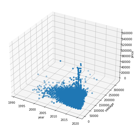
Before you start learning, let's check the characteristics of the dataset (displacement, mileage, price against year of manufacture).
in [8]:
|
fig = plt.figure(figsize=(16, 8)) plt.subplots_adjust(wspace=0.4, hspace=0.4) ax1 = fig.add_subplot(2, 2, 1) ax1.scatter(all_brand['engineSize'], all_brand['price']) ax1.set_title('All_Brand', size =, 15) ax1.set_xlabel('engineSize') ax1.set_ylabel('price') ax2 = fig.add_subplot(2, 2, 2) ax2.scatter(all_brand['mileage'], all_brand['price']) ax2.set_title('All_Brand', size =, 15) ax2.set_xlabel('mileage') ax2.set_ylabel('price') ax3 = fig.add_subplot(2, 2, 3) ax3.scatter(all_brand['year'], all_brand['price']) ax3.set_title('All_Brand', size =, 15) ax3.set_xlabel('year') ax3.set_ylabel('price') plt.show() |

Visualizing with 3D graph.
in [9]:
|
fig = plt.figure(figsize=(16, 8)) plt.subplots_adjust(wspace=0.4, hspace=0.4) ax4 = fig.add_subplot(1, 1, 1, projection = '3d') ax4.set_xlabel('year') ax4.set_ylabel('mileage') ax4.set_zlabel('price') ax4.scatter(all_brand['year'], all_brand['mileage'], all_brand['price']) plt.show() |
Extracting input data x and output data y from DataFrame.
in [10]:
|
y = all_brand[['price']] x = all_brand[['year', 'mileage', 'engineSize']] |
Separating data for learning and testing.
in [11]:
|
x_train, x_test, y_train, y_test = train_test_split(x, y, test_size=0.1, random_state=13) np_y_train = y_train.to_numpy().ravel(); np_y_test = y_test.to_numpy().ravel() print(x_train) print(np_y_train) |
| all_brand.head() |
Out[6]:
| year | mileage | engineSize | |
| 385 | 2016 | 29302 | 1.4 |
| 11592 | 2014 | 55861 | 1.2 |
| 10258 | 2019 | 6682 | 1.0 |
| 3094 | 2017 | 15116 | 2.0 |
| 1622 | 2017 | 59383 | 1.0 |
| ... | ... | ... | ... |
| 6141 | 2013 | 46800 | 1.0 |
| 7914 | 2019 | 4250 | 2.0 |
| 3730 | 2017 | 23185 | 1.4 |
| 1453 | 2017 | 11627 | 1.0 |
| 3994 | 2017 | 36659 | 1.6 |
[97426 rows x 3 columns]
[ 7000 5561 17991 ... 9220 12591 9990]
Starting the Frovedis server.
in [12]:
|
FrovedisServer.initialize("mpirun -np 6 {}".format(os.environ['FROVEDIS_SERVER'])) |
'[ID: 1] FrovedisServer (Hostname: handson02, Port: 36630) has been initialized with 6 MPI processes.'
in [13]:
|
for i in [0.1, 0.01, 0.001]: for j in [100, 250, 500,750]: gbt = gbt.fix(x_train, np_train) gbt = GradientBoostingRegressor(learning_rate=i, n_estimators=j) print("predict output for GradientBoostingRegressor: learning_rate={}, n_estimators={}".format(i, j)) mse = mean_squared_erro(np_y_test, gbt.predict(x_test)) print("The mean squared error (MSE) on test set: {:.4f}".format(mse)) pred2 = gbt.predict(x_test) print("Accuracy on training set: %.3f" % gbt.score(x_train, np_y_train)) print("Accuracy on test set: %.3f" % gbt.score(x_test, np_y_test)) print("==============================================") |
The mean squared error (MSE) on test set: 16958423.9092
Accuracy on training set: 0.824
Accuracy on test set: 0.823
==============================================
predict output for GradientBoostingRegressor: learning_rate=0.1, n_estimators=250
The mean squared error (MSE) on test set: 16773506.7649
Accuracy on training set: 0.828
Accuracy on test set: 0.825
==============================================
predict output for GradientBoostingRegressor: learning_rate=0.1, n_estimators=500
The mean squared error (MSE) on test set: 16731805.4272
Accuracy on training set: 0.830
Accuracy on test set: 0.826
==============================================
predict output for GradientBoostingRegressor: learning_rate=0.1, n_estimators=750
The mean squared error (MSE) on test set: 16756739.8292
Accuracy on training set: 0.831
Accuracy on test set: 0.825
==============================================
predict output for GradientBoostingRegressor: learning_rate=0.01, n_estimators=100
The mean squared error (MSE) on test set: 21688407.8670
Accuracy on training set: 0.771
Accuracy on test set: 0.774
==============================================
predict output for GradientBoostingRegressor: learning_rate=0.01, n_estimators=250
The mean squared error (MSE) on test set: 18676782.5213
Accuracy on training set: 0.803
Accuracy on test set: 0.805
==============================================
predict output for GradientBoostingRegressor: learning_rate=0.01, n_estimators=500
The mean squared error (MSE) on test set: 17588219.4446
Accuracy on training set: 0.815
Accuracy on test set: 0.817
==============================================
predict output for GradientBoostingRegressor: learning_rate=0.01, n_estimators=750
The mean squared error (MSE) on test set: 17225708.6052
Accuracy on training set: 0.820
Accuracy on test set: 0.820
==============================================
predict output for GradientBoostingRegressor: learning_rate=0.001, n_estimators=100
The mean squared error (MSE) on test set: 28317220.1012
Accuracy on training set: 0.703
Accuracy on test set: 0.705
==============================================
predict output for GradientBoostingRegressor: learning_rate=0.001, n_estimators=250
The mean squared error (MSE) on test set: 26177106.2856
Accuracy on training set: 0.725
Accuracy on test set: 0.727
==============================================
predict output for GradientBoostingRegressor: learning_rate=0.001, n_estimators=500
The mean squared error (MSE) on test set: 24060917.7513
Accuracy on training set: 0.747
Accuracy on test set: 0.749
==============================================
predict output for GradientBoostingRegressor: learning_rate=0.001, n_estimators=750
The mean squared error (MSE) on test set: 22547915.3948
Accuracy on training set: 0.762
Accuracy on test set: 0.765
==============================================
in [14]:
|
x_test.loc[:,['price']] = pred2 x_test.head() |
Out[14]:
| year | mileage | engineSize | prize | |
| 10035 | 2019 | 3052 | 1.0 | 14715.109924 |
| 9238 | 2019 | 14310 | 1.0 | 14483.300719 |
| 8404 | 2019 | 13723 | 1.4 | 15100.060242 |
| 3077 | 2020 | 1500 | 2.0 | 29945.443639 |
| 16655 | 2017 | 19128 | 1.0 | 11491.146581 |
Learning and testing with the parameters that give the most accurate results.
in [15]:
|
gbt = GradientBoostingRegressor(learning_rate=0.1, n_estimators=0, ) gbt = gbt.fit(x_train, np_y_train) print("predict output for GradientBoostingRegressor: learning_rate={}, n_estimators={}".format(i, j)) mse = mean_squared_error(np_y_test, gbt.predict(x_test) print("The mean squared error (MSE) on test set: {:.4f}".format(mse)) pred2 = gbt.predict(x_test) print("The best accuracy on test set: %.3f" % gbt.score(x_terst, np_y_test)) |
predict output for GradientBoostingRegressor: learning_rate=0.001, n_estimators=750
The mean squared error (MSE) on test set: 16731805.4272
The best accuracy on training set: 0.830
The best accuracy on test set: 0.826
Displaying the parameter list of the training model.
in [16]:
|
print(gbt.get_params()) |
in [17]:
|
FrovedisServer.shut_down() |
As shown in this column, changing individual parameters to check test accuracy and degree of overfitting is one way to obtain the best learning model. Repeated training of large datasets is time consuming.
By using the processing parallel algorithms of SX-Aurora TSUBASA and Frovedis, it is possible to create a high-performance learning model at a lower cost.